How To Draw A Density Curve
How To Draw A Density Curve - The value “7” occurs 5. The probability of any event is the area under the density curve and above the values of x that. If we created a simple histogram to display the relative frequencies of each value, it would look like this: Analyzing skew, median, mean and height of a density curve. A brief review of frequency histograms and. Density (d) is a physical property found by dividing the mass of an object by its volume. The easiest way to create a density plot in matplotlib is to use the kdeplot () function from the seaborn visualization library: We use a density curve to describe the distribution of a continuous variable. Library(tidyverse) tibble(x = rnorm(10000, mean = 34, sd = 4.5)) |> ggplot(aes(x)) +. So the simplest way i could come up with is: The value “7” occurs 5. Learn about the importance of density curves and their properties. Data = [value1, value2, value3,. However you can find the gaussian probability density function in scipy.stats. If we created a simple histogram to display the relative frequencies of each value, it would look like this: Regardless of the sample size, density is always constant. Learn how to add a density or a normal curve over an histogram in base r with the density and lines functions You can use rnorm to create a sample distribution for a given mean and sd, then ggplot: The easiest way to create a density plot in matplotlib is to use the kdeplot () function from the seaborn visualization library: Density (d) is a physical property found by dividing the mass of an object by its volume. So the simplest way i could come up with is: The value “7” occurs 5. And now, we combined the equations d=m/v and pv=nrt to get a whole new mod. Data = [value1, value2, value3,. Density (d) is a physical property found by dividing the mass of an object by its volume. A brief review of frequency histograms and. The probability of any event is the area under the density curve and above the values of x that. The easiest way to create a density plot in matplotlib is to use the kdeplot () function from the seaborn visualization library: The value “7” occurs 5. Data = [value1, value2, value3,. However you can find the gaussian probability density function in scipy.stats. An introduction to density curves for visualizing distributions. Suppose we have the following dataset that shows the height of 20 different plants (in inches) in a certain field: Both of these concepts will be explained in this video. The probability distribution of a continuous random variable x is described. Suppose we have the following dataset that shows the height of 20 different plants (in inches) in a certain field: Library(tidyverse) tibble(x = rnorm(10000, mean = 34, sd = 4.5)) |> ggplot(aes(x)) +. A brief review of frequency histograms and. And now, we combined the equations d=m/v and pv=nrt to get a whole new mod. Both of these concepts will. The probability distribution of a continuous random variable x is described by a density curve. There are two common ways to create a distribution plot in python: An introduction to density curves for visualizing distributions. Learn about the importance of density curves and their properties. Both of these concepts will be explained in this video. So the simplest way i could come up with is: An introduction to density curves for visualizing distributions. Regardless of the sample size, density is always constant. Learn about the importance of density curves and their properties. We use a density curve to describe the distribution of a continuous variable. We use a density curve to describe the distribution of a continuous variable. However you can find the gaussian probability density function in scipy.stats. An introduction to density curves for visualizing distributions. Start practicing—and saving your progress—now: Library(tidyverse) tibble(x = rnorm(10000, mean = 34, sd = 4.5)) |> ggplot(aes(x)) +. If we created a simple histogram to display the relative frequencies of each value, it would look like this: Suppose we have the following dataset that shows the height of 20 different plants (in inches) in a certain field: The easiest way to create a density plot in matplotlib is to use the kdeplot () function from the seaborn visualization. Gases already have a lot going on, whizzing around like that. Density (d) is a physical property found by dividing the mass of an object by its volume. The probability distribution of a continuous random variable x is described by a density curve. Learn about the importance of density curves and their properties. Library(tidyverse) tibble(x = rnorm(10000, mean = 34,. Suppose we have the following dataset that shows the height of 20 different plants (in inches) in a certain field: You can use rnorm to create a sample distribution for a given mean and sd, then ggplot: Draw a density histogram for the resulting data. However you can find the gaussian probability density function in scipy.stats. There are two common. We use a density curve to describe the distribution of a continuous variable. Start practicing—and saving your progress—now: Learn how to add a density or a normal curve over an histogram in base r with the density and lines functions A brief review of frequency histograms and. Note that color controls the fill color of the bars, ec controls. The value “7” occurs 5. Analyzing skew, median, mean and height of a density curve. Data = [value1, value2, value3,. And now, we combined the equations d=m/v and pv=nrt to get a whole new mod. The probability of any event is the area under the density curve and above the values of x that. Density (d) is a physical property found by dividing the mass of an object by its volume. Draw a density histogram for the resulting data. You can use rnorm to create a sample distribution for a given mean and sd, then ggplot: Gases already have a lot going on, whizzing around like that. The easiest way to create a density plot in matplotlib is to use the kdeplot () function from the seaborn visualization library: On top of the histogram plot, overlay the theoretical exponential probability density function, that is, f(t) = 3e−3t f (t) = 3 e − 3 t for t> 0 t>.Solved Consider the density curve below. What is the height of the

SOLVEDDensity curves Sketch a density curve that might describe a
Density curve for uncensored real D2. Download Scientific Diagram
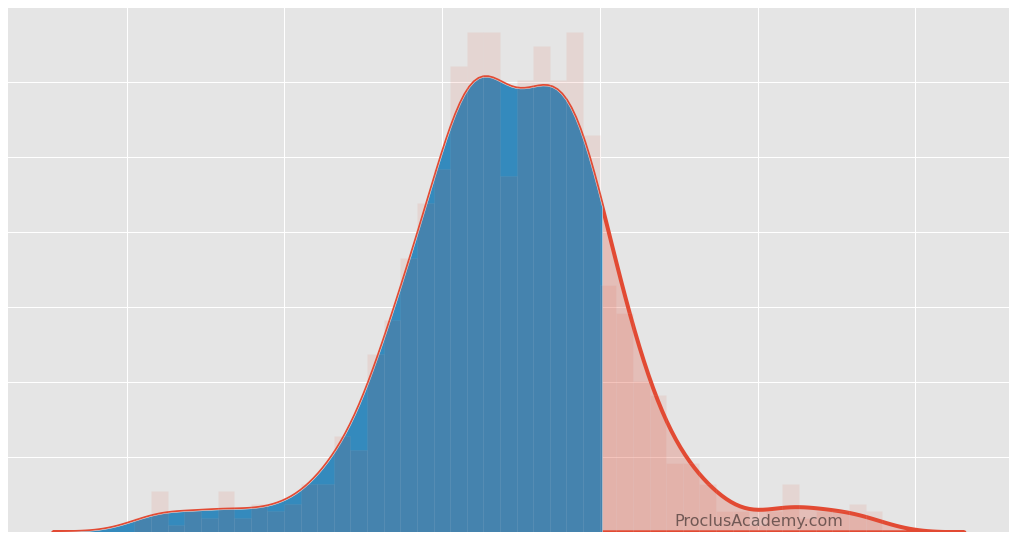
Area Under Density Curve How to Visualize and Calculate Using Python
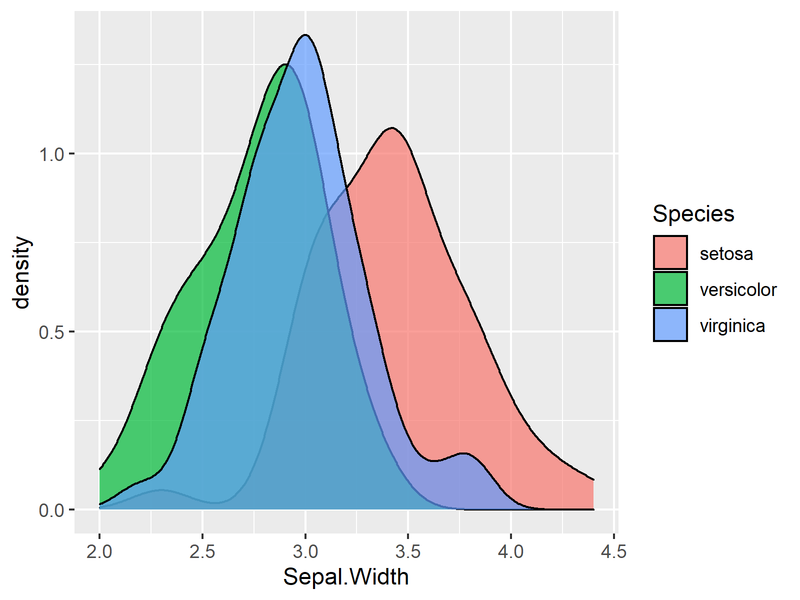
R Draw Several ggplot2 Density Plots in Same Graphic (Example Code)
Density curve for uncensored real D1. Download Scientific Diagram
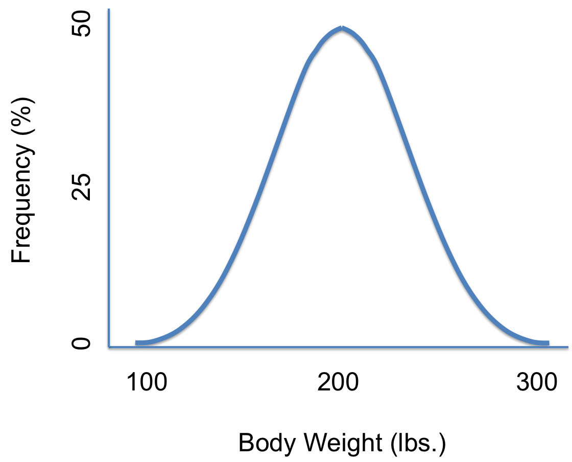
Density Curve Examples
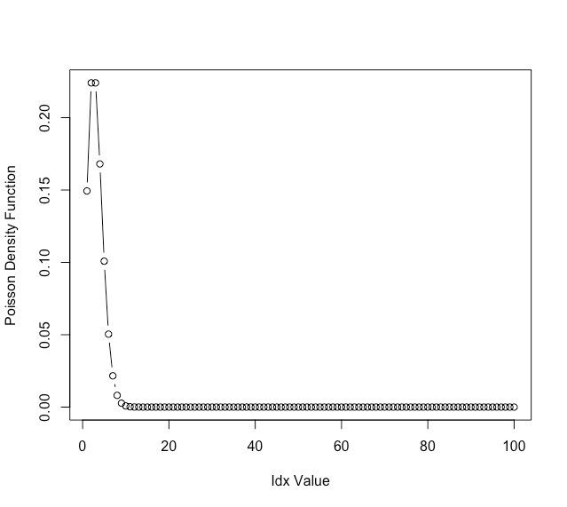
How to Draw Poisson Density Curve in R?
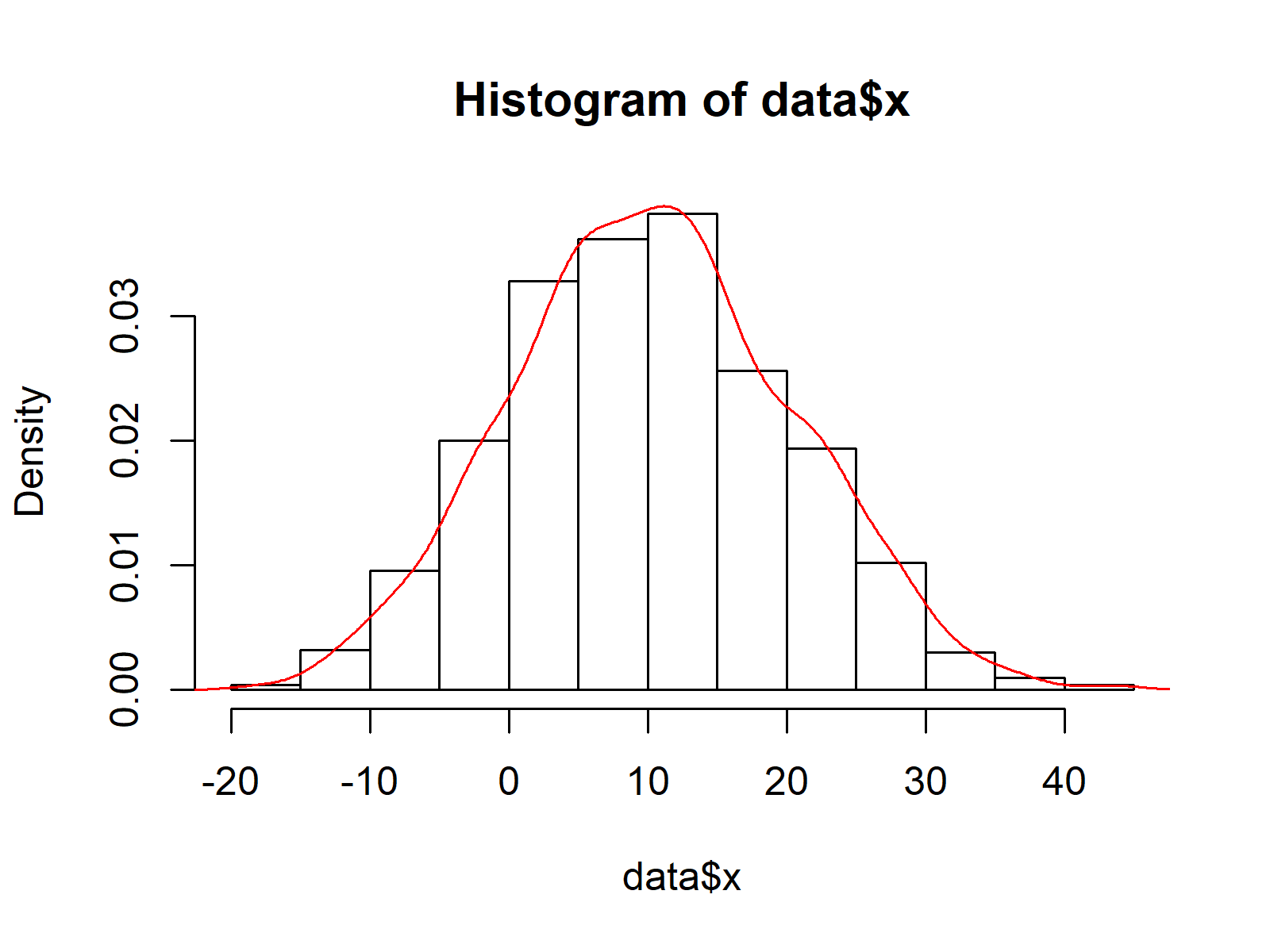
Overlay Histogram with Fitted Density Curve Base R & ggplot2 Example
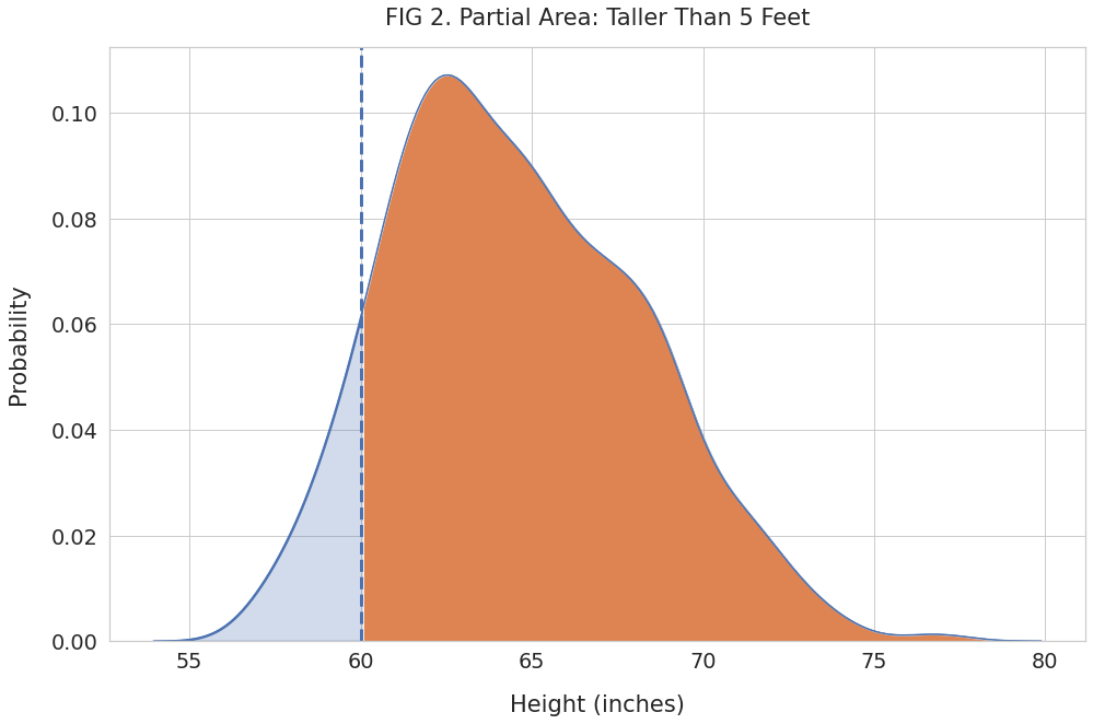
Area Under Density Curve How to Visualize and Calculate Using Python
Library(Tidyverse) Tibble(X = Rnorm(10000, Mean = 34, Sd = 4.5)) |> Ggplot(Aes(X)) +.
Regardless Of The Sample Size, Density Is Always Constant.
Both Of These Concepts Will Be Explained In This Video.
If We Created A Simple Histogram To Display The Relative Frequencies Of Each Value, It Would Look Like This:
Related Post: