Draw Prior From 1/Sigma Square
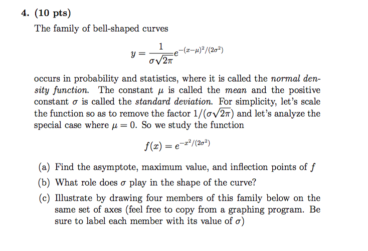
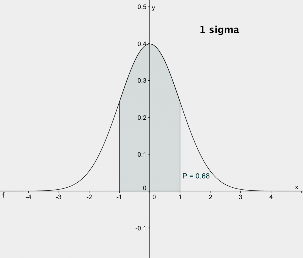
Draw Prior From 1/Sigma Square - I'm reading bayesian core, and the authors state that a jeffreys prior $\pi(\beta,\sigma^2|x)\propto\frac{1}{\sigma^2}$ corresponds to a flat prior on. So, we can choose what we mentioned when we called conjugate priors, priors such that the posteriors are going to be of. For a normal likelihood, the jeffreys prior is \(g(\sigma) \propto 1/\sigma\). See the docs for gamma and inverse gamma distributions. This is often useful as a way to see if the sampling distribution or prior we. We may care about making predictions before we even see any data. For now, assume we have only one measurement (n=. Target += normal_lpdf(first_variable | first_means, first_sigmas); Specify a prior for mu and a different prior for sigma square. For simplicity we will treat τ as known initially. See the docs for gamma and inverse gamma distributions. This is often useful as a way to see if the sampling distribution or prior we. 1.1 posterior for single measurement (n= 1) we want to put together the prior (2) and the likelihood (1) to get the posterior ( jx). It also coincides with the. For a normal likelihood, the jeffreys prior is \(g(\sigma) \propto 1/\sigma\). So, we can choose what we mentioned when we called conjugate priors, priors such that the posteriors are going to be of. For a normal likelihood, the jeffreys prior is \(g(\sigma) \propto 1/\sigma\). I'm reading bayesian core, and the authors state that a jeffreys prior $\pi(\beta,\sigma^2|x)\propto\frac{1}{\sigma^2}$ corresponds to a flat prior on. That means that the priors for parameters \(\mu\) and \(\sigma\) are independent and that. For simplification let’s express the precision (inverse variance) as a new parameter, \(\phi = 1/\sigma^2\). For simplicity we will treat τ as known initially. Target += normal_lpdf(second_variable | second_means + rhos.* first_sigmas./ second_sigmas.*. This distribution is called uninformative because it is. We may care about making predictions before we even see any data. Target += normal_lpdf(first_variable | first_means, first_sigmas); I'm reading bayesian core, and the authors state that a jeffreys prior $\pi(\beta,\sigma^2|x)\propto\frac{1}{\sigma^2}$ corresponds to a flat prior on. Specify a prior for mu and a different prior for sigma square. For simplification let’s express the precision (inverse variance) as a new parameter, \(\phi = 1/\sigma^2\). That means that the priors for parameters \(\mu\) and \(\sigma\) are independent and that. Specify a prior for mu and a different prior for sigma square. That means that the priors for parameters \(\mu\) and \(\sigma\) are independent and that parameter \(\mu\) should. For now, assume we have only one measurement (n=. See the docs for gamma and inverse gamma distributions. Target += normal_lpdf(first_variable | first_means, first_sigmas); These use the same parametrizations as defined in the 'stan' documentation. This is often useful as a way to see if the sampling distribution or prior we. I'm reading bayesian core, and the authors state that a jeffreys prior $\pi(\beta,\sigma^2|x)\propto\frac{1}{\sigma^2}$ corresponds to a flat prior on. We may care about making predictions before we even see any data. For simplification. We may care about making predictions before we even see any data. That means that the priors for parameters \(\mu\) and \(\sigma\) are independent and that. This is often useful as a way to see if the sampling distribution or prior we. For now, assume we have only one measurement (n=. So, we can choose what we mentioned when we. Specify a prior for mu and a different prior for sigma square. Target += normal_lpdf(first_variable | first_means, first_sigmas); This is often useful as a way to see if the sampling distribution or prior we. That means that the priors for parameters \(\mu\) and \(\sigma\) are independent and that parameter \(\mu\) should. This distribution is called uninformative because it is. For a normal likelihood, the jeffreys prior is \(g(\sigma) \propto 1/\sigma\). So, we can choose what we mentioned when we called conjugate priors, priors such that the posteriors are going to be of. This distribution is called uninformative because it is. Specify a prior for mu and a different prior for sigma square. That means that the priors for parameters. Target += normal_lpdf(first_variable | first_means, first_sigmas); So, we can choose what we mentioned when we called conjugate priors, priors such that the posteriors are going to be of. Specify a prior for mu and a different prior for sigma square. Target += normal_lpdf(second_variable | second_means + rhos.* first_sigmas./ second_sigmas.*. For now, assume we have only one measurement (n=. So, we can choose what we mentioned when we called conjugate priors, priors such that the posteriors are going to be of. 1.1 posterior for single measurement (n= 1) we want to put together the prior (2) and the likelihood (1) to get the posterior ( jx). These use the same parametrizations as defined in the 'stan' documentation. See the. That means that the priors for parameters \(\mu\) and \(\sigma\) are independent and that. For now, assume we have only one measurement (n=. For a normal likelihood, the jeffreys prior is \(g(\sigma) \propto 1/\sigma\). For simplification let’s express the precision (inverse variance) as a new parameter, \(\phi = 1/\sigma^2\). See the docs for gamma and inverse gamma distributions. You can see easily that if $\beta \rightarrow 0$ and $\alpha \rightarrow 0$ then the inverse gamma will approach the jeffreys prior. See the docs for gamma and inverse gamma distributions. For simplicity we will treat τ as known initially. These use the same parametrizations as defined in the 'stan' documentation. Then the conjugate prior for \(\phi\), \[\begin{equation} \phi \sim. For simplification let’s express the precision (inverse variance) as a new parameter, \(\phi = 1/\sigma^2\). So, we can choose what we mentioned when we called conjugate priors, priors such that the posteriors are going to be of. See the docs for gamma and inverse gamma distributions. It also coincides with the. We may care about making predictions before we even see any data. Target += normal_lpdf(first_variable | first_means, first_sigmas); For a normal likelihood, the jeffreys prior is \(g(\sigma) \propto 1/\sigma\). Specify a prior for mu and a different prior for sigma square. 1.1 posterior for single measurement (n= 1) we want to put together the prior (2) and the likelihood (1) to get the posterior ( jx). That means that the priors for parameters \(\mu\) and \(\sigma\) are independent and that parameter \(\mu\) should. That means that the priors for parameters \(\mu\) and \(\sigma\) are independent and that.
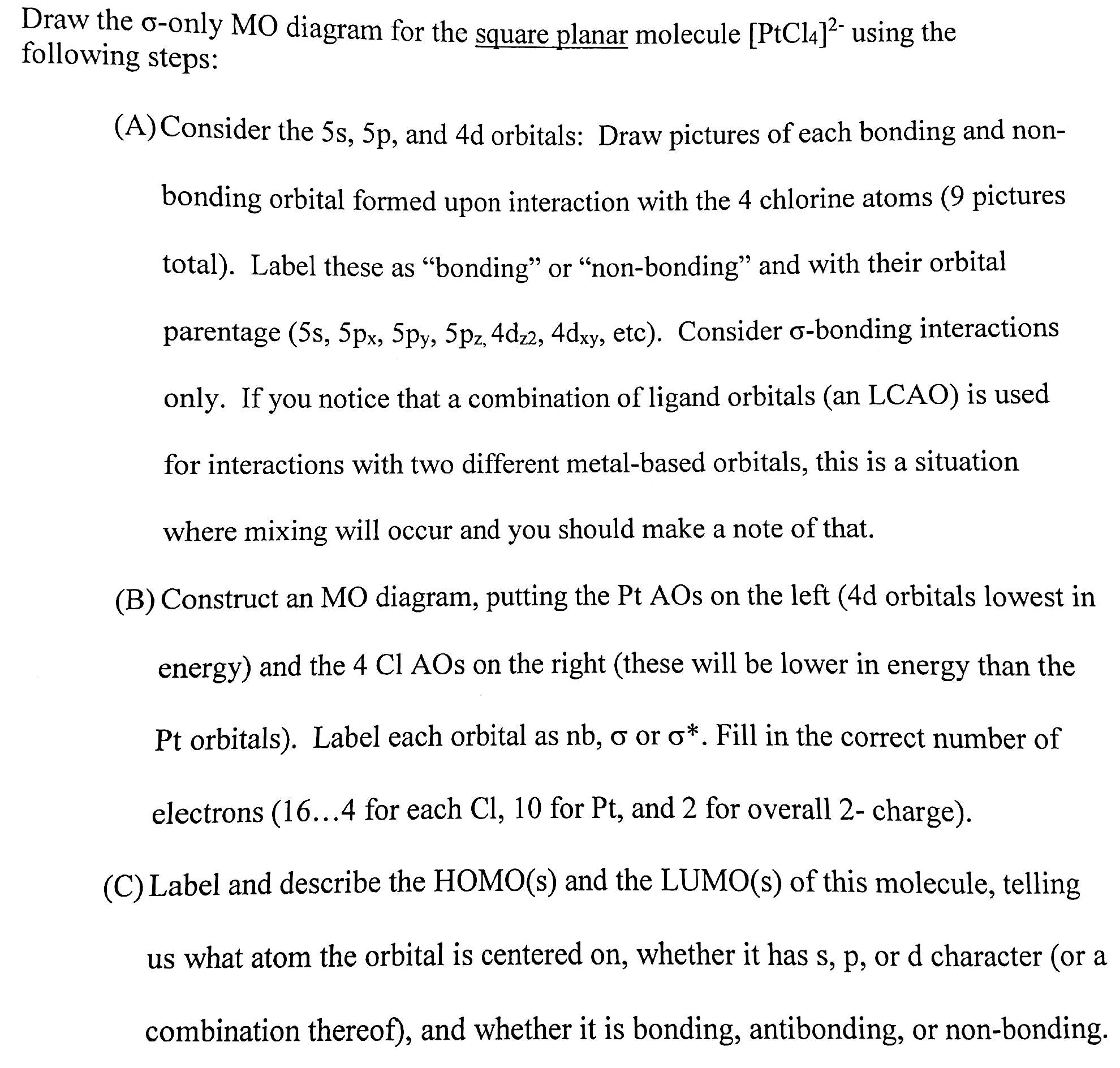
OneClass Draw the sigmaonly MO diagram for the square planar molecule
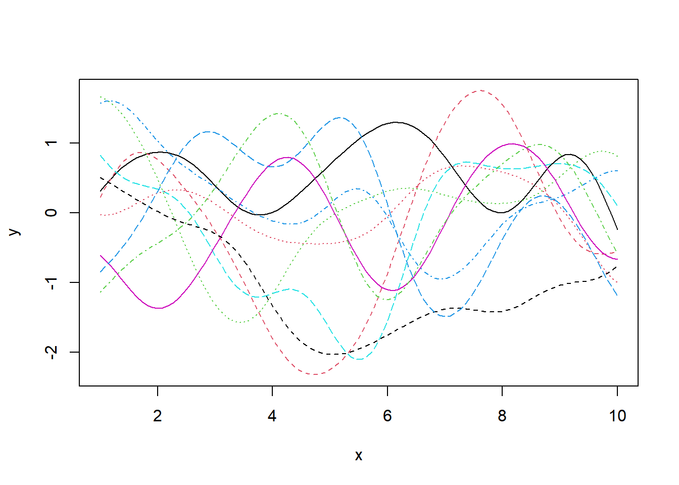
Derivatives of a Gaussian Process Herb Susmann
Read "Notes on Uniform Distribution and Normal
PPT Neural Firing PowerPoint Presentation, free download ID1780167

Why is X\hat{\beta} regarded as y in multiple linear regression
OneClass Draw the sigmaonly MO diagram for the square planar molecule
The family of bellshaped curves y = 1/sigma square
Lecture 14

Lecture 11 Estimation of Sigma Square YouTube

Evalaute Sum of Series with Square in Sigma Notation for a Quadratic
For A Normal Likelihood, The Jeffreys Prior Is \(G(\Sigma) \Propto 1/\Sigma\).
For Now, Assume We Have Only One Measurement (N=.
Target += Normal_Lpdf(Second_Variable | Second_Means + Rhos.* First_Sigmas./ Second_Sigmas.*.
This Distribution Is Called Uninformative Because It Is.
Related Post: